Methodology
How the numbers on the dashboard are made
Every number the dashboard shows is computed live by the models described here: the methods, how each figure was measured, and the limits of what the models cover.
Figures are produced by the evaluation scripts in the repository, linked at the end.
1. What you are looking at
An Asian option is a contract whose payout depends on the average price of a stock over the contract's life rather than only its final price, and there is no exact formula for its fair value. The standard way to price one is to simulate a large number of possible futures and average the payout, which is accurate but slow: the 400,000-path reference behind the benchmark table below takes 946 milliseconds for a single price in the committed benchmark run, and a trading desk needs thousands of prices and their risk sensitivities refreshed continuously. This project trains a neural network on those simulated prices so that it learns the pricing function itself, and it then answers in about 4 milliseconds in the same run, 236 times faster, with a measured error of 1.3 basis points of strike against 200,000-path references. Because the network is a smooth function, its risk sensitivities (the Greeks) come out as exact derivatives of the network in the same call, instead of by nudging each input and re-pricing; delta and vega are fitted to, and measured against, pathwise Monte Carlo derivatives, and section 3 gives their error. The dashboard shows the network's answer next to a fresh simulation with its confidence interval so you can check it yourself.
2. How it works
One model for every strike
An Asian call's price scales linearly in spot and strike: multiply both by the same factor and
the price scales with them. So the network only learns the unit-strike price as a function of
moneyness, maturity, volatility and rate, f(S/K, T, σ, r), and any contract is
priced as K · f(S/K, T, σ, r). One model covers every strike exactly, and puts
come from Asian put-call parity, which is also exact. The test suite checks parity for both
the Monte Carlo engine and the surrogate.
The network, the training signal, and the ensemble
The pricer is a residual multilayer perceptron with SiLU activations and LayerNorm, about 134k parameters. Smooth activations matter because the Greeks are derivatives of the network; a ReLU network would have zero gamma almost everywhere. Five independently initialized networks are averaged as a deep ensemble, which lowers error, and the Greeks average cleanly through the mean.
Training follows differential machine learning (Huge and Savine, 2020): the pathwise delta and vega are computed on the same Monte Carlo paths that produce each price, for almost no extra cost, and the network is fit to the prices and their derivatives together in a variance-normalized loss. A controlled ablation at the same sample budget, prices only versus the differential loss, cut delta error about 3x and vega error about 4x. The served model was trained on 500,000 labels of 5,000 paths each for 400 epochs. Label generation runs on the GPU in float64 at 0.85 G path-steps/s on an RTX 5080, so the full set takes 148 s instead of roughly 80 minutes on CPU; float64 is not optional, because the same kernel at float32 with identical seeds injects 10.03 bps of price RMSE at 5,000 paths.
Greeks by automatic differentiation
All five Greeks are exact derivatives of the network obtained by automatic differentiation, not finite differences. The test suite checks four of them: delta, vega and theta against finite-difference perturbations of the network, and rho against the closed-form parity derivative at three contracts, to 1e-6. Gamma is measured on the same 600 held-out contracts against a conditional-Monte-Carlo reference: the arithmetic average is linear in the spot, so gamma is the discounted density of the scaled average at the strike, and conditioning on the first increment gives that density in closed form with no kernel and no bandwidth (it reproduces Black-Scholes gamma to machine precision when the contract has one fixing). The ensemble's gamma error is 140 × 10−4 RMSE per unit of (S/K)2, of which the reference's own Monte Carlo noise accounts for 50 × 10−4 RMS, with standard errors taken over antithetic pairs. Where gamma is large (Black-Scholes-scale gamma above 0.5, 222 contracts) the median relative error is 0.46 % against a median reference standard error of 0.35 %, so the comparison resolves gamma to about that floor. The error concentrates at small σ√T, the same hinge region the arbitrage audit identifies: 356 × 10−4 RMSE below σ√T = 0.1 (where the reference's own noise is 104 × 10−4) against 75 above 0.2. They are quoted per share of the underlying: delta per $1 of spot, gamma per $1 squared, vega and rho per point of volatility and of rate (1 % = 1 point), and theta per trading day, 252 to a year. Every maturity on the site is in the same trading days, so decay per day times days to expiry is the premium of the contract as quoted. Theta is the derivative with respect to maturity, and an Asian's 50 fixing dates are spread over its life, so shortening the maturity moves the averaging window as well as the time left: it is a tenor sensitivity, not calendar decay on a fixed schedule. A price alone costs about 4 ms in the benchmark below. Price plus all five Greeks costs roughly twelve times that, because gamma needs a second backward pass through each of the five ensemble members. Serving is CPU-only in every code path here, and the dashboard reports the latency of each request it served.
Monte Carlo: antithetic sampling and a geometric control variate
The reference engine, which generates the training labels and the live comparison price on
the dashboard, uses antithetic sampling with a geometric-Asian control variate (Kemna and
Vorst, 1990). The geometric-average option has a closed-form price, so the simulation error
on it can be measured and subtracted from the arithmetic estimate. On an at-the-money one-year
contract at 20% volatility and a 5% rate, measured as the ratio of empirical standard deviations
across 300 seeded replications with antithetic sampling in both arms, the control variate cuts
the standard error by about 24x: 22x to 26x at 5,000 paths and 23x to 24x at 20,000, over two
sets of 300 replications. The factor is specific to that contract: the same protocol at 5,000
paths gives 48x to 55x on a three-month at-the-money contract at 20% volatility, and 5x to 10x
at three other points of the trained box (the one-year contract at 60% volatility; spot 80
against a strike of 100 at
three months and 30% volatility; spot 130 against a strike of 100 at two years and 70%
volatility). scripts/variance_reduction.py reproduces these figures into
docs/variance_reduction.json. On the dashboard the
benchmark switches regime automatically: Asian under geometric Brownian motion above 12
trading days to expiry, rough Bergomi at or below.
Same-day expiry: a rough Bergomi surrogate with exact Volterra simulation
Very short-dated option smiles show a power-law skew that classical models cannot reproduce,
so a separate five-member ensemble serves maturities of 12 trading days or less, trained on a
rough Bergomi Monte Carlo engine. The driver is the Riemann-Liouville Volterra process of
Bayer, Friz and Gatheral (2016), W̃_t = √(2H) ∫₀ᵗ (t−s)^(H−½) dW_s, simulated
exactly from the joint Gaussian law of the driving Brownian motion and the Volterra
integral; the scheme is verified against quadrature to 5.4e-08 and against 400,000 draws.
The served ensemble is trained on the dynamics of a live SPY calibration: on 2026-08-20 the
calibrator fitted η = 3.66, ρ = −0.63 and H = 0.26 jointly with the forward
variance to 618 live mid quotes across seven expiries at 1.57 vol points of implied-vol
RMSE, the fit passed the quality gate, and the checkpoint records that provenance in its
own metadata. Its ensemble validation RMSE is 3.3 bps of strike against its 20,000-path
training labels; re-priced against 400,000-path rough Bergomi references at its hardest
smiles (one to five days at 10% vol) the price RMSE is 1.9 to 3.8 bps.
The rough-volatility signature: how fast the skew steepens
The market-facing reason to use rough volatility for short-dated options is the term
structure of the at-the-money skew: rough models predict that the skew
ψ(T) = dσimp/dk steepens like a power law
TH−½ as expiry approaches, which classical stochastic
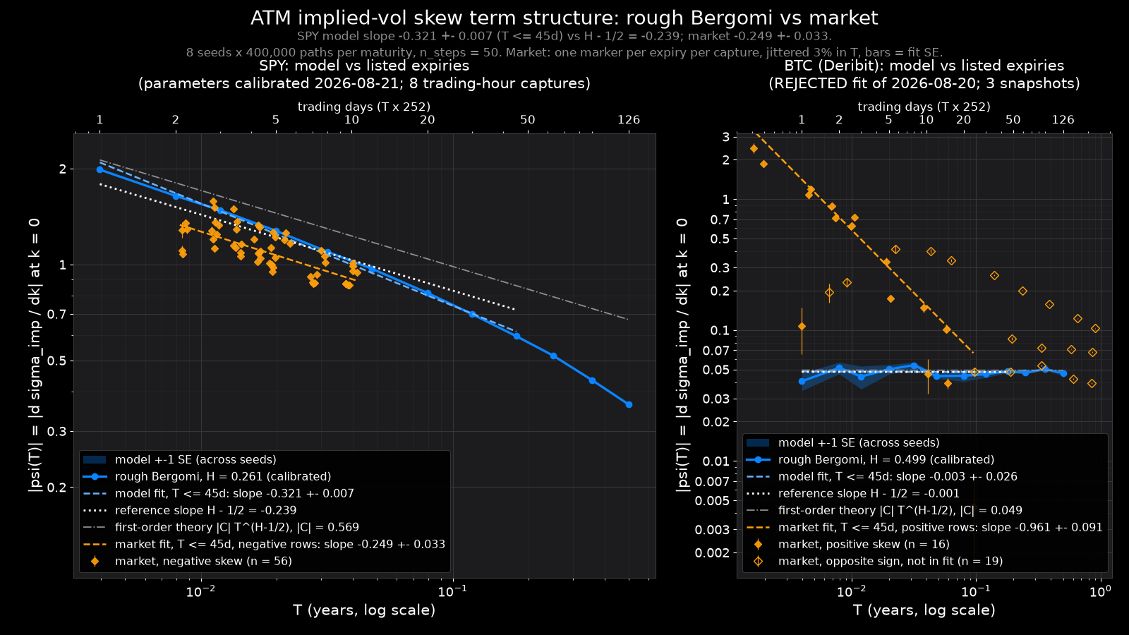
volatility cannot reproduce. Measured from the committed SPY option captures (8 captures across
two trading days, 7 expiries each, 56 local-quadratic fits between 2 and 10 trading days), the
market exponent is −0.249 ± 0.033, against H − ½ = −0.239
for H = 0.261, the value in the SPY calibration record the experiment reads (the served 0DTE
checkpoint's own fit has H = 0.255, whose H − ½ = −0.245 is also
within one standard error of the market). The model side is measured the same way, by Monte Carlo with 8 seeds
× 400,000 paths per maturity: at that fit's vol-of-vol (η = 3.9) the model's skew is
steeper than the asymptotic law (exponent −0.321 ± 0.007) because ηTH is
already 0.9 at one day, while at η = 0.5 the same engine returns −0.233 ± 0.011
with an amplitude within 0.4% of the first-order theory. Bitcoin, for contrast, shows no power
law at all: its front-month skew is positive.
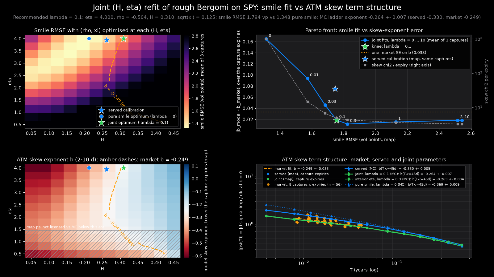
scripts/atm_skew_term_structure.py.The term structure also identifies the parameters better than a single day's smile. A smile calibration never sees it explicitly, and buys short-dated curvature most cheaply with more vol-of-vol, which is why that fit's η sits at its bound. Refitting (H, η, ρ, ξ) jointly against the smiles and the per-expiry ATM skew, on a 12 × 12 profile over (H, η) with the remaining parameters optimised at every cell, moves the optimum to H = 0.31, ρ = −0.50 and a forward vol of 12.5 % (bootstrap: H 0.308 ± 0.011) and puts the Monte Carlo skew exponent at −0.264 ± 0.007, within half a market standard error of −0.249, for a cost of 0.45 vol points of smile fit (1.31 to 1.76). A solution with η off its bound reaches the same exponent for 0.15 vol points more. The served short-dated model was trained on an earlier accepted fit (H = 0.255) and is unchanged; the refit is recorded as an analysis artifact.
scripts/joint_skew_refit.py.An arbitrage-free implied-volatility surface
A network that outputs option prices can be smooth and still wrong in a way no market
allows: nothing stops it from pricing a butterfly spread below zero or a longer option below
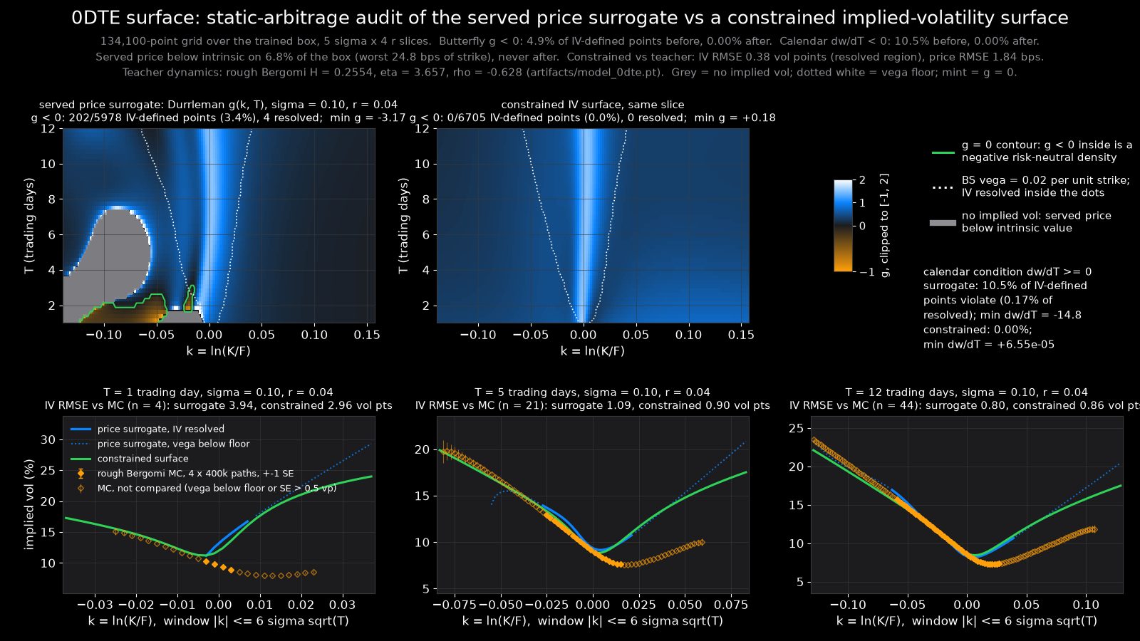
a shorter one. Audited by automatic differentiation on 134,100 points across its trained
box, the 0DTE pricing ensemble does exactly that at the edges: its implied total variance
violates the Durrleman butterfly condition g(k) ≥ 0 on 4.9% of the points
where an implied vol exists and the calendar condition on 10.5%, concentrated deep
in-the-money at very low volatility and one to two days to expiry; inside the region
where its implied vol is resolved by vega, violations are rare (0.06% and 0.18%). The
surface served on the dashboard is a second, small network (12,929 parameters) that
models total implied variance as a positive output times a Black-Scholes prior and is
trained against the ensemble with autograd penalties on both conditions and on the
large-moneyness slope, following Ackerer, Tagasovska and Vatter (2020). On the same
134,100 points it has zero violations (minimum g +0.072, minimum
∂w/∂T +6.5×10⁻⁵), never prices below intrinsic value, and
reproduces the ensemble to 0.22 vol points where the implied vol is resolved. It inherits
the ensemble's short-end error against a 400,000-path Monte Carlo of the true dynamics
(up to 3 vol points at one day and 10% vol), so it is arbitrage-free, not more accurate.
The dashboard evaluates both conditions on the displayed grid for every setting of
σ and r.
scripts/no_arbitrage_surface.py.Heston as the classical reference
Every neural number above is checked against Monte Carlo, whose error is statistical. A
semi-analytic reference has none: backend/quant/heston.py prices European
options under Heston (1993) by the COS method of Fang and Oosterlee (2008) with the
characteristic function in the numerically stable form of Albrecher and coauthors, and
reproduces the published reference value 5.785155450 to 8×10⁻⁹,
satisfies put-call parity to 10−11, recovers Black-Scholes in the
zero-vol-of-vol limit to 10−13, and agrees with an independent Euler Monte
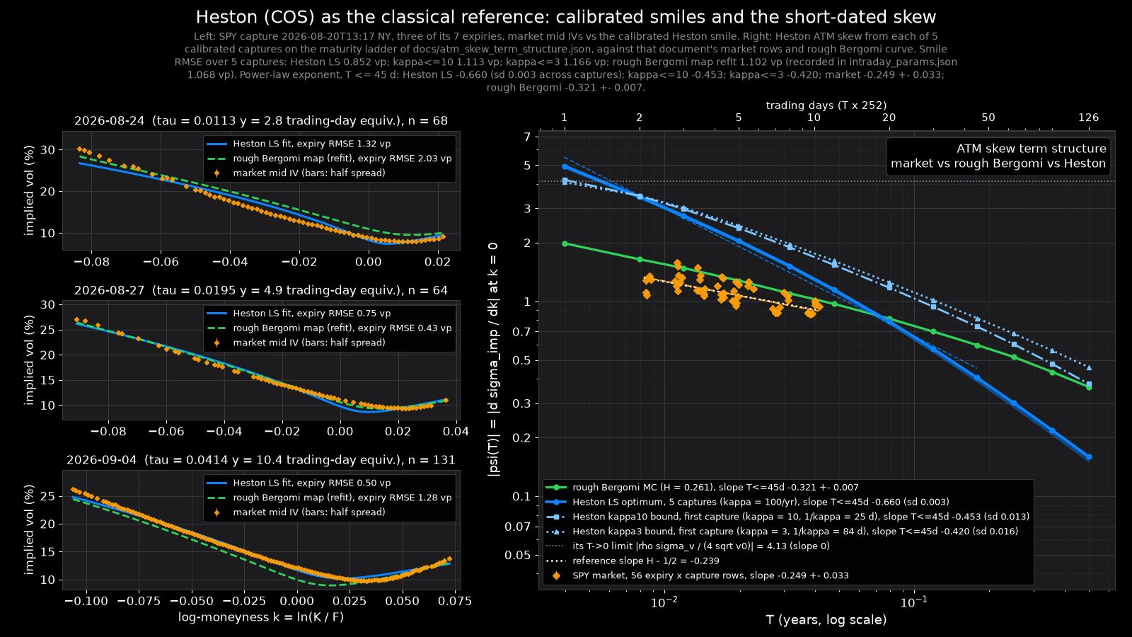
Carlo within one standard error, pricing a 100-strike smile in 3.6 ms. Calibrated to the same
SPY captures as the rough Bergomi map, Heston fits the two-to-ten-day smiles slightly better
(0.85 versus 1.10 vol points RMSE over five captures) but only by pushing the mean-reversion
speed to its 100-per-year bound with a vol-of-variance near 4.7, and its at-the-money skew
then steepens into expiry with exponent −0.66 against the market's −0.25, twice
too fast; with mean reversion capped at 10 per year the fit worsens to 1.11 vol points and
the exponent is −0.45. Textbook Heston parameters give the classical flat short-dated
skew (exponent near 0). A single-day smile does not identify the model; the term structure
of the skew does.
scripts/heston_reference.py.Deep hedging and the CVaR objective
Following Buehler and coauthors (2019), a policy network maps the hedging state to a position
and is trained to minimize the 95% conditional value at risk of the terminal loss, with
transaction costs inside the objective. The Hedging tab simulates 15,000 paths (five seeded
blocks of 3,000) of hedging a short 30-day at-the-money call to expiry, and shows the learned policy's
profit-and-loss distribution against a vol-matched Black-Scholes delta hedge and a cost-aware
Whalley-Wilmott no-trade band on the same paths. On Black-Scholes dynamics the learned policy
does not beat either baseline on tail risk; under rough volatility with transaction costs it
reaches a lower tail loss than the delta hedge, mostly by trading less, which is the
experiment below. Replayed over eight years of real SPY
and BTC daily history with only ex-ante information, the default hedger.pt
checkpoint (a policy trained on the GAN market simulator, which the dashboard does not
serve) keeps its cost efficiency (better mean P&L at 50 bp of cost on 69% of SPY
windows, trading about half as much as delta) but not its tail advantage. Neither served
policy has been replayed on history; the paired tables and that provenance are in
docs/hedging_real_paths.md.
Deep hedging under rough volatility, jumps and costs
On Black-Scholes paths the market is complete and a delta hedge is close to optimal, so a learned
policy has little to win there. The dashboard's Deep Hedging tab therefore simulates the
SPY-calibrated rough Bergomi model with compensated jumps (H = 0.25, ρ = −0.55, an
incomplete market with stochastic rough volatility correlated with spot) and runs three hedgers
on identical paths: the learned policy, a vol-matched Black-Scholes delta, and a
Whalley-Wilmott no-trade band tuned in the baseline's favour. A fourth, a linear-regression
hedge in the style of Ruf and Wang, is reported in
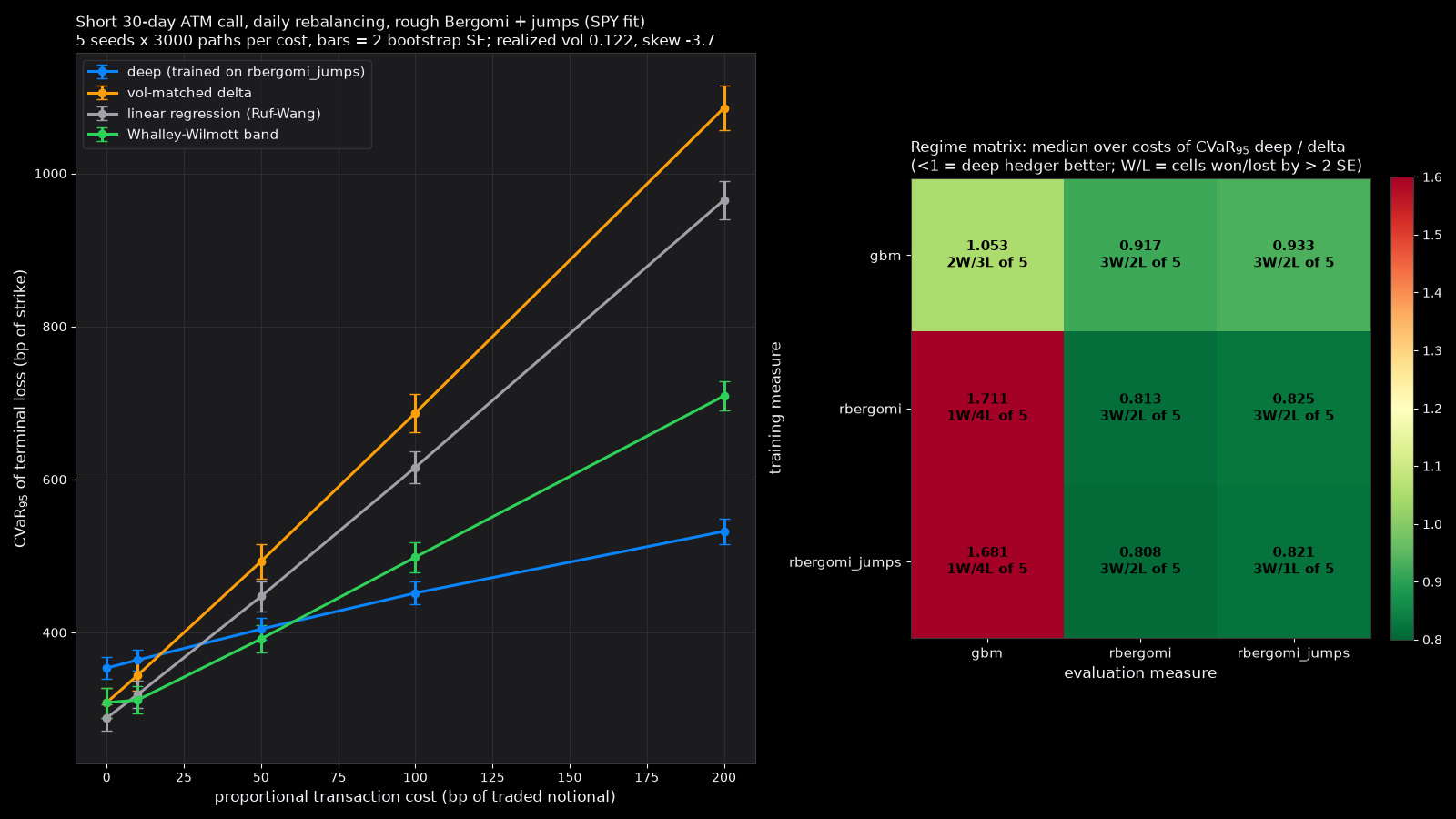
docs/deep_hedging_regimes.md. Across 15,000 paths per cost the learned policy's tail loss crosses below the
delta hedge at 50 bp of proportional cost (CVaR95 404 ± 7 versus
493 ± 11 bp of strike) and below the Whalley-Wilmott band at 100 bp
(452 ± 8 versus 498 ± 10), reaching half the delta hedge's tail loss at 200 bp.
It does so by holding about 0.23 less than the Black-Scholes delta, the under-hedge that
minimum-variance theory predicts when spot and volatility are negatively correlated, and by
trading a third of the delta hedge's turnover. Most of that gap is the smaller commission
bill rather than a better-shaped tail: CVaR95 splits exactly into the mean loss
and the tail about that mean, and at 50 bp of cost 78.5 of the 88.5 bp advantage over the
delta hedge is mean and 10.0 bp is tail shape. On demeaned tail alone the
Whalley-Wilmott band is ahead below 200 bp. The same policy evaluated on Black-Scholes paths
loses, as it should: the edge is specific to the dynamics it was trained on.
The ± figures are bootstrap standard errors over those 15,000 evaluation paths, for one
trained policy per training measure: the policies trained under geometric Brownian motion,
rough Bergomi and rough Bergomi with jumps all use training seed 21. They do not include the
spread from retraining the network. That spread is measured separately, with the dashboard's
own hedge run at 50 bp: policies trained on four seeds and scored on two sets of evaluation
paths put the advantage over the delta hedge between 48 and 99 bp of strike
(scripts/hedger_seed_spread.py, docs/deep_hedging_seed_spread.json).
scripts/deep_hedging_regimes.py.Explainability by integrated gradients
The feature-attribution panel runs Integrated Gradients through the ensemble against an at-the-money baseline, so each input is credited with its share of the price difference from that baseline. The completeness check, that the attributions sum to the price difference, is reported alongside, so a bad attribution shows up as a visible residual rather than disappearing into the chart.
Real market data
Everything above runs on simulated data. The exception is a live Deribit option chain: 836 BTC instruments across 12 expiries, fetched from public endpoints with no API key and committed as a snapshot so the diagnostics run offline. Reading the coin-denominated premium on the per-expiry forward and inverting Black-76 reproduces Deribit's own published mark IV to a median of 0.0028 vol points; reading it as a dollar price instead gives 4.62 vol points where the truth is 32.88, wrong by 7.1x and still a smooth, plausible surface. Of 51 static-arbitrage violations that appear on mid prices, zero are executable once the actual bid-ask has to be crossed.
3. Results
Everything here is measured, not asserted. The evaluation script prices a held-out test set against high-precision Monte Carlo references; the model is never scored against its own noisy training labels, because that overstates the error (by 2.4x on the 0DTE model). The test set is a fresh Latin-hypercube draw from the same parameter box as the training set and is labelled by the same simulator, so these figures are interpolation error inside the trained box, not evidence of generalisation beyond it.
| Quantity | Error (RMSE) |
|---|---|
| Price | 1.3 bps of strike |
| Delta | 7.3e-4, per $1 of spot |
| Vega | 1.3e-3 of strike, per 1.00 of σ |
| Method | RMSE | Bias | p95 abs err |
|---|---|---|---|
| Neural ensemble | 1.395 bps | +0.308 | 3.312 |
| Levy (1992) moment matching | 38.911 bps | +17.662 | 99.335 |
| Curran (1994), exact threshold | 2.347 bps | −1.038 | 4.859 |
| Monte Carlo, 200k paths | (reference) | n/a | n/a |
Against Levy the ensemble is 27.9x more accurate over the full trained box, with a 95% interval of 22.9 to 33.5 from a paired bootstrap over the 300 points. The ratio is an average over a box where volatility runs to 80%. Levy's error is a bias that grows with σ²T, so the ratio depends on where the box is sampled: by σ band it is 1.8, 14.0 and 37.8, and at a more typical σ = 0.25 the margin narrows to about 5x, 0.72 against 3.65 bps of mean absolute error. The one regime where Levy wins is where the true price is below 1 bp of strike (0.049 versus 0.396 bps over 19 of the 300 points), a consequence of the Softplus output floor at prices near zero.
Curran's (1994) conditioning approximation is a rigorous lower bound on the arithmetic-average price and the stronger baseline at typical volatilities. It has the lower RMSE for σ below 0.55, and the ensemble has it from 0.55 to 0.80 (1.725 against 3.969 bps), where the gap between the lower bound and the true price widens with σ²T. On a 36-cell grid at σ = 0.25 Curran is 6.9x more accurate than the ensemble at about a tenth of the latency.
| Method | Mean abs err | Max abs err | Bias | Latency |
|---|---|---|---|---|
| Neural ensemble | 0.719 bps | 2.045 | +0.712 | 4.00 ms |
| Curran (1994), exact threshold | 0.104 bps | 0.345 | −0.104 | 399 µs |
| Levy (1992) moment matching | 3.654 bps | 13.282 | +2.028 | 312 µs |
| Monte Carlo, 400k paths | (reference) | SE ≤ 0.207 | n/a | 946.06 ms |
So the case for the surrogate on a Black-Scholes Asian is not price accuracy. It is the rest of the package: all five Greeks by automatic differentiation in the same call, batch throughput that the dashboard measures live on whichever machine is serving, and a training recipe that needs no geometric-conditioning trick and therefore carries over to dynamics where no such closed form exists, which is exactly how the short-dated rough Bergomi ensemble is built. Curran is a geometric-Brownian-motion result on a fixed averaging schedule and does not extend to rough volatility.
| Operation | Cost |
|---|---|
| Single price | 4.00 ms |
| Single price plus all five Greeks | about 12x a price-only call |
| 400,000-path Monte Carlo reference, one price | 946.06 ms |
| Quantity | Value |
|---|---|
| Calibration fit, 618 live SPY quotes across 7 expiries | 1.57 vol points IV RMSE |
| Ensemble validation RMSE against 20,000-path training labels | 3.3 bps of strike |
| Price RMSE against 4 × 400,000-path references, six smiles at 1/5/12 days and 10%/20% vol | 0.79 to 3.76 bps |
| Largest single-strike error on those smiles | 14.4 bps |
| Policy | Beats vol-matched delta | Median ratio | Beats Whalley-Wilmott |
|---|---|---|---|
| Trained on the GAN market simulator | 2 / 12 | 1.469 | 0 / 12 |
| Trained on GBM (in-sample) | 5 / 12 | 1.085 | 1 / 12 |
| Cost | Delta hedge | Whalley-Wilmott | Linear regression | Deep policy | Deep / delta |
|---|---|---|---|---|---|
| 0 bp | 308 ± 10 | 308 ± 10 | 288 ± 9 | 354 ± 7 | 1.15 |
| 10 bp | 344 ± 10 | 312 ± 9 | 319 ± 9 | 364 ± 7 | 1.06 |
| 50 bp | 493 ± 11 | 392 ± 9 | 447 ± 10 | 404 ± 7 | 0.82 |
| 100 bp | 687 ± 12 | 498 ± 10 | 616 ± 11 | 452 ± 8 | 0.66 |
| 200 bp | 1086 ± 15 | 709 ± 10 | 965 ± 13 | 532 ± 9 | 0.49 |
| Series | Exponent | Reference H − ½ |
|---|---|---|
| SPY listed expiries, 8 captures × 7 expiries | −0.249 ± 0.033 | −0.239 |
| Rough Bergomi, latest SPY fit (η = 3.9) | −0.321 ± 0.007 | −0.239 |
| Rough Bergomi, η = 0.5 (asymptotic regime) | −0.233 ± 0.011 | −0.239 |
| Rough Bergomi, joint (H, η) refit against smiles + skew (H = 0.31) | −0.264 ± 0.007 | −0.190 |
| Heston, least-squares optimum (κ at the 100/yr bound) | −0.660 (sd 0.003 across captures) | n/a |
| Heston, κ ≤ 10/yr | −0.453 (sd 0.013) | n/a |
| Model | RMSE (mean over captures) |
|---|---|
| Heston, least squares (5 parameters) | 0.85 |
| Heston, κ ≤ 10/yr | 1.11 |
| Rough Bergomi, pricing-map calibration (4 parameters) | 1.10 |
| Surface | Butterfly g < 0 | Calendar ∂w/∂T < 0 | Price below intrinsic | IV RMSE vs ensemble |
|---|---|---|---|---|
| 0DTE pricing ensemble (prices) | 4.9% | 10.5% | 6.8% | n/a |
| Constrained implied-vol surface (served) | 0 | 0 | 0 | 0.22 vol pts |
The advantage above is specific to rough volatility with costs. On Black-Scholes paths the market is complete and the classical baselines hold: across a 12-cell sweep of training and evaluation measures on those paths, the learned policy loses to a vol-matched delta hedge in 7 cells and to the Whalley-Wilmott band in 11. Even under rough volatility the band remains the stronger baseline until costs reach 100 bp. The dashboard runs all three hedgers on the same paths and ranks them by tail loss for the run in front of you.
Because they share paths, the dashboard compares them the way the table above does: paired. One bootstrap resample of the paths is drawn per replicate and every hedger is scored on it, so the common path risk cancels inside each replicate and what is left is the sampling error of the comparison itself. Combining two separate error bars instead, hypot(SEa, SEb), would assume the hedgers were independent, and they are the opposite of independent: a path that is bad for one is usually bad for all three. On the served run at 50 bp the paired errors are 20-58 % smaller than the unpaired formula claims, which changes what the page is entitled to say. The learned policy beats the vol-matched delta hedge by $0.94 ± 0.11 and the Ruf-Wang linear hedge by $0.14 ± 0.06, both intervals clear of zero. Against the Whalley-Wilmott band it is $0.10 ± 0.08 behind, an interval that still contains zero: the band leads on the point estimate and wins about 89 % of resamples, and that is as far as 15,000 paths will carry it. Both the Hedging tab and the risk summary read the same intervals, so they cannot disagree about what this run separates.
| Check | Result |
|---|---|
| Black-76 inversion versus Deribit's published mark IV | median 0.0028 vol pts |
| Quotes flagged and dropped | 289 of 836 |
| IV bid-ask on surviving quotes | median 1.36, p95 9.79 vol pts |
| Static-arbitrage violations on mid / executable through the spread | 51 / 0 |
| Parity-implied forward versus listed future, 12 expiries | median under 1 bp |
4. Scope
- This is a research and portfolio project, not production trading infrastructure. Nothing here is investment advice.
- The Asian pricer takes a single flat volatility rather than a full surface and carries no arbitrage constraint of its own, and the short-dated pricing ensemble is not arbitrage-free by construction either. The short-dated implied-volatility surface on the dashboard is the separately trained constrained network that is, and the two are compared above.
- The rough Bergomi model has constant parameters: η, ρ and H are fitted jointly to one smile and none of them varies with maturity, so one fit covers the short-dated range and longer expiries would need their own. The served short-dated checkpoint was trained on a single calibration to SPY quotes captured on 20 August 2026 and is not refit as the market moves. Fitting H against the skew term structure as well moves it (see the joint refit above), but the served model was not retrained on that result.
- The deep hedger's advantage is regime-specific. On Black-Scholes paths the classical baselines win; under rough volatility with transaction costs it beats the delta hedge, and the Whalley-Wilmott band from 100 bp; on eight years of real SPY and BTC daily history it keeps its cost efficiency (better mean P&L at 50 bp of cost on 69% of SPY windows) but not its tail advantage. The GAN market simulator used in early training is not a reliable evaluation measure, so no result is reported on it. Each simulated result comes from one trained policy per measure, and its error bars cover the evaluation paths, not retraining.
- The served pricer favours price accuracy: its delta and vega are 5.9% and 1.2% less accurate than an alternative head that prices slightly worse. A service hedging off these Greeks should weigh that differently from a service pricing with them.
- The second-order Greeks are not hedging-grade. An autograd audit of the served Asian ensemble over 120,800 points of its own trained box finds gamma negative on 18.6% of it and vega negative on 28.1%, concentrated where the average is nearly deterministic and the true price is a hinge with no curvature to reproduce; inside the region where a reference vega resolves at all, 0.06% of convexity checks fail and every other condition is clean. Gamma's held-out error against the conditional-density reference is measured above; no hedging experiment in this project runs on the surrogate's own Greeks, since the hedging comparisons use a Black-Scholes delta throughout.
- The absolute price RMSE moves with the test draw (1.301 to 1.488 bps across four independent draws); only paired comparisons on identical points and references are treated as meaningful.
- Market data for the ticker feature comes from yfinance, which is retail-grade and has stale or missing quotes. The Deribit chain is a committed snapshot, not a live feed.
- The live demo runs on a small always-on instance; the Monte Carlo engines simulate in fixed-size blocks of paths so the whole service runs within 512 MB of memory.
5. Links
- The live dashboard: Quote, Hedge, Live and Desk note.
- Source code on GitHub: the README, the trained checkpoints, and the evaluation scripts.
- docs/deep_hedging_regimes.md: the deep hedging experiment under rough volatility, jumps and costs, every cell with standard errors.
- docs/approximation_benchmark.md: the surrogate against the Levy (1992) and Curran (1994) closed forms, cell by cell, with the protocol and the reference standard errors.
- docs/atm_skew_term_structure.md: the skew term-structure measurement, model and market.
- docs/joint_skew_refit.md: the joint (H, η) refit against smiles and skew term structure, with the Pareto front and Monte Carlo validation.
- docs/no_arbitrage_surface.md: the static-arbitrage audit and the constrained implied-vol surface.
- docs/asian_arbitrage_audit.md: the static-arbitrage audit of the Asian pricer, in price space, over its own trained box.
- docs/heston_reference.md: the Heston COS pricer, its verification, calibration and skew term structure.
- docs/hedging_findings.md: the Black-Scholes deep hedging evaluation.
- docs/hedging_real_paths.md: the same hedgers replayed over real SPY and BTC price history.
- docs/real_market_data.md: the Deribit chain, its conventions and its diagnostics.
- DEPLOY.md: hosting notes.
Research tool. Prices come from neural surrogates trained on simulated data and are not investment advice. Built with PyTorch, FastAPI and Plotly. MIT licensed.